![]()
Lesson 9 Data Science Libraries
Pragmatic AI Labs
![]()
This notebook was produced by Pragmatic AI Labs. You can continue learning about these topics by:
- Buying a copy of Pragmatic AI: An Introduction to Cloud-Based Machine Learning
- Reading an online copy of Pragmatic AI:Pragmatic AI: An Introduction to Cloud-Based Machine Learning
- Watching video Essential Machine Learning and AI with Python and Jupyter Notebook-Video-SafariOnline on Safari Books Online.
- Watching video AWS Certified Machine Learning-Speciality
- Purchasing video Essential Machine Learning and AI with Python and Jupyter Notebook- Purchase Video
- Viewing more content at noahgift.com
Setup Tasks
Install Latest Plotly
import plotly
plotly.__version__
'3.6.1'
!pip uninstall -q -y plotly
!pip install plotly==3.6.0
!pip install -q --upgrade cufflinks
Collecting plotly==3.6.0
[?25l Downloading https://files.pythonhosted.org/packages/4d/59/63a5a05532a67b1c49283e8b7885bbe55454a1eef8443e97a7479bb9964b/plotly-3.6.0.tar.gz (31.1MB)
[K 100% |████████████████████████████████| 31.1MB 999kB/s
[?25hRequirement already satisfied: decorator>=4.0.6 in /usr/local/lib/python3.6/dist-packages (from plotly==3.6.0) (4.3.2)
Requirement already satisfied: nbformat>=4.2 in /usr/local/lib/python3.6/dist-packages (from plotly==3.6.0) (4.4.0)
Requirement already satisfied: pytz in /usr/local/lib/python3.6/dist-packages (from plotly==3.6.0) (2018.9)
Requirement already satisfied: requests in /usr/local/lib/python3.6/dist-packages (from plotly==3.6.0) (2.18.4)
Collecting retrying>=1.3.3 (from plotly==3.6.0)
Downloading https://files.pythonhosted.org/packages/44/ef/beae4b4ef80902f22e3af073397f079c96969c69b2c7d52a57ea9ae61c9d/retrying-1.3.3.tar.gz
Requirement already satisfied: six in /usr/local/lib/python3.6/dist-packages (from plotly==3.6.0) (1.11.0)
Requirement already satisfied: traitlets>=4.1 in /usr/local/lib/python3.6/dist-packages (from nbformat>=4.2->plotly==3.6.0) (4.3.2)
Requirement already satisfied: jupyter-core in /usr/local/lib/python3.6/dist-packages (from nbformat>=4.2->plotly==3.6.0) (4.4.0)
Requirement already satisfied: ipython-genutils in /usr/local/lib/python3.6/dist-packages (from nbformat>=4.2->plotly==3.6.0) (0.2.0)
Requirement already satisfied: jsonschema!=2.5.0,>=2.4 in /usr/local/lib/python3.6/dist-packages (from nbformat>=4.2->plotly==3.6.0) (2.6.0)
Requirement already satisfied: idna<2.7,>=2.5 in /usr/local/lib/python3.6/dist-packages (from requests->plotly==3.6.0) (2.6)
Requirement already satisfied: certifi>=2017.4.17 in /usr/local/lib/python3.6/dist-packages (from requests->plotly==3.6.0) (2018.11.29)
Requirement already satisfied: chardet<3.1.0,>=3.0.2 in /usr/local/lib/python3.6/dist-packages (from requests->plotly==3.6.0) (3.0.4)
Requirement already satisfied: urllib3<1.23,>=1.21.1 in /usr/local/lib/python3.6/dist-packages (from requests->plotly==3.6.0) (1.22)
Building wheels for collected packages: plotly, retrying
Building wheel for plotly (setup.py) ... [?25ldone
[?25h Stored in directory: /root/.cache/pip/wheels/67/0b/29/08c7f5caed2d1ac446db982ff607b326d49bfa0bd3a67ef8c7
Building wheel for retrying (setup.py) ... [?25ldone
[?25h Stored in directory: /root/.cache/pip/wheels/d7/a9/33/acc7b709e2a35caa7d4cae442f6fe6fbf2c43f80823d46460c
Successfully built plotly retrying
Installing collected packages: retrying, plotly
Successfully installed plotly-3.6.0 retrying-1.3.3
import plotly
plotly.__version__
'3.6.0'
def enable_plotly_in_cell():
import IPython
from plotly.offline import init_notebook_mode
display(IPython.core.display.HTML('''
<script src="/static/components/requirejs/require.js"></script>
'''))
init_notebook_mode(connected=False)
9.1 Learn numpy
References
What is numpy?
- Low level multi-dimensional array library
- A programmers Excel
- The building blocks for many key Python libraries:
- Pandas
- Sklearn
- Tensorflow
Hello World Numpy Workflow
import numpy as np
Make an array
a = np.arange(6).reshape(2, 3)
Print shape
a.shape
(2, 3)
Print size
a.size
6
Print type
a.dtype.name
'int64'
Print contents
a
array([[0, 1, 2],
[3, 4, 5]])
Create an Array
One Dimensional Array
a = np.array([2,4,6,8])
print(f"Shape {a.shape}")
print(f"Content: {a}")
Shape (4,)
Content: [2 4 6 8]
Two Dimensional Array
a = np.array([(2,4,6,8),(20,40,60,80)])
print(f"Shape: {a.shape}")
print(f"Content: {a}")
Shape: (2, 4)
Content: [[ 2 4 6 8]
[20 40 60 80]]
Create Sequence of Numbers
a = np.arange(1,20)
print(f"Shape: {a.shape}")
print(f"Content: {a}")
Shape: (19,)
Content: [ 1 2 3 4 5 6 7 8 9 10 11 12 13 14 15 16 17 18 19]
Create empty multi-dimensional array
a = np.zeros( (2,3) )
print(f"Shape: {a.shape}")
print(f"Content: {a}")
Shape: (2, 3)
Content: [[0. 0. 0.]
[0. 0. 0.]]
Applied Numpy
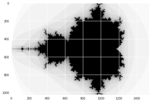
Numpy Non-GPU Mandelbrot
import numpy as np
from pylab import imshow, show
from timeit import default_timer as timer
def mandel(x, y, max_iters):
"""
Given the real and imaginary parts of a complex number,
determine if it is a candidate for membership in the Mandelbrot
set given a fixed number of iterations.
"""
c = complex(x, y)
z = 0.0j
for i in range(max_iters):
z = z*z + c
if (z.real*z.real + z.imag*z.imag) >= 4:
return i
return max_iters
def create_fractal(min_x, max_x, min_y, max_y, image, iters):
height = image.shape[0]
width = image.shape[1]
pixel_size_x = (max_x - min_x) / width
pixel_size_y = (max_y - min_y) / height
for x in range(width):
real = min_x + x * pixel_size_x
for y in range(height):
imag = min_y + y * pixel_size_y
color = mandel(real, imag, iters)
image[y, x] = color
image = np.zeros((1024, 1536), dtype = np.uint8)
start = timer()
create_fractal(-2.0, 1.0, -1.0, 1.0, image, 20)
dt = timer() - start
print("Mandelbrot created in %f s" % dt)
imshow(image)
show()
Mandelbrot created in 5.650793 s
Numba Mandelbrot
Numba is LLVM JIT support for Python
from numba import autojit
import numpy as np
from timeit import default_timer as timer
@autojit
def mandel(x, y, max_iters):
"""
Given the real and imaginary parts of a complex number,
determine if it is a candidate for membership in the Mandelbrot
set given a fixed number of iterations.
"""
c = complex(x, y)
z = 0.0j
for i in range(max_iters):
z = z*z + c
if (z.real*z.real + z.imag*z.imag) >= 4:
return i
return max_iters
@autojit
def create_fractal(min_x, max_x, min_y, max_y, image, iters):
height = image.shape[0]
width = image.shape[1]
pixel_size_x = (max_x - min_x) / width
pixel_size_y = (max_y - min_y) / height
for x in range(width):
real = min_x + x * pixel_size_x
for y in range(height):
imag = min_y + y * pixel_size_y
color = mandel(real, imag, iters)
image[y, x] = color
image = np.zeros((1024, 1536), dtype = np.uint8)
start = timer()
create_fractal(-2.0, 1.0, -1.0, 1.0, image, 20)
dt = timer() - start
print("Mandelbrot created in %f s" % dt)
imshow(image)
show()
Mandelbrot created in 0.361222 s

Cuda-Numpy
CUDA Install
!/usr/local/cuda/bin/nvcc --version
nvcc: NVIDIA (R) Cuda compiler driver
Copyright (c) 2005-2018 NVIDIA Corporation
Built on Sat_Aug_25_21:08:01_CDT_2018
Cuda compilation tools, release 10.0, V10.0.130
CUDA GPU Mandelbrot
from numba import cuda
from numba import *
mandel_gpu = cuda.jit(restype=uint32, argtypes=[f8, f8, uint32], device=True)(mandel)
@cuda.jit(argtypes=[f8, f8, f8, f8, uint8[:,:], uint32])
def mandel_kernel(min_x, max_x, min_y, max_y, image, iters):
height = image.shape[0]
width = image.shape[1]
pixel_size_x = (max_x - min_x) / width
pixel_size_y = (max_y - min_y) / height
startX, startY = cuda.grid(2)
gridX = cuda.gridDim.x * cuda.blockDim.x;
gridY = cuda.gridDim.y * cuda.blockDim.y;
for x in range(startX, width, gridX):
real = min_x + x * pixel_size_x
for y in range(startY, height, gridY):
imag = min_y + y * pixel_size_y
image[y, x] = mandel_gpu(real, imag, iters)
---------------------------------------------------------------------------
OSError Traceback (most recent call last)
/usr/local/lib/python3.6/dist-packages/numba/cuda/cudadrv/nvvm.py in __new__(cls)
110 try:
--> 111 inst.driver = open_cudalib('nvvm', ccc=True)
112 except OSError as e:
/usr/local/lib/python3.6/dist-packages/numba/cuda/cudadrv/libs.py in open_cudalib(lib, ccc)
47 if path is None:
---> 48 raise OSError('library %s not found' % lib)
49 if ccc:
OSError: library nvvm not found
During handling of the above exception, another exception occurred:
NvvmSupportError Traceback (most recent call last)
<ipython-input-34-dff031d8ec9d> in <module>()
2 sys.path.append('/usr/local/lib/python3.6/site-packages/')
3
----> 4 @cuda.jit(argtypes=[f8, f8, f8, f8, uint8[:,:], uint32])
5 def mandel_kernel(min_x, max_x, min_y, max_y, image, iters):
6 height = image.shape[0]
/usr/local/lib/python3.6/dist-packages/numba/cuda/decorators.py in kernel_jit(func)
94 # Force compilation for the current context
95 if bind:
---> 96 kernel.bind()
97
98 return kernel
/usr/local/lib/python3.6/dist-packages/numba/cuda/compiler.py in bind(self)
498 Force binding to current CUDA context
499 """
--> 500 self._func.get()
501
502 @property
/usr/local/lib/python3.6/dist-packages/numba/cuda/compiler.py in get(self)
376 cufunc = self.cache.get(device.id)
377 if cufunc is None:
--> 378 ptx = self.ptx.get()
379
380 # Link
/usr/local/lib/python3.6/dist-packages/numba/cuda/compiler.py in get(self)
348 arch = nvvm.get_arch_option(*cc)
349 ptx = nvvm.llvm_to_ptx(self.llvmir, opt=3, arch=arch,
--> 350 **self._extra_options)
351 self.cache[cc] = ptx
352 if config.DUMP_ASSEMBLY:
/usr/local/lib/python3.6/dist-packages/numba/cuda/cudadrv/nvvm.py in llvm_to_ptx(llvmir, **opts)
472
473 def llvm_to_ptx(llvmir, **opts):
--> 474 cu = CompilationUnit()
475 libdevice = LibDevice(arch=opts.get('arch', 'compute_20'))
476 # New LLVM generate a shorthand for datalayout that NVVM does not know
/usr/local/lib/python3.6/dist-packages/numba/cuda/cudadrv/nvvm.py in __init__(self)
144 class CompilationUnit(object):
145 def __init__(self):
--> 146 self.driver = NVVM()
147 self._handle = nvvm_program()
148 err = self.driver.nvvmCreateProgram(byref(self._handle))
/usr/local/lib/python3.6/dist-packages/numba/cuda/cudadrv/nvvm.py in __new__(cls)
114 errmsg = ("libNVVM cannot be found. Do `conda install "
115 "cudatoolkit`:\n%s")
--> 116 raise NvvmSupportError(errmsg % e)
117
118 # Find & populate functions
NvvmSupportError: libNVVM cannot be found. Do `conda install cudatoolkit`:
library nvvm not found
---------------------------------------------------------------------------
NOTE: If your import is failing due to a missing package, you can
manually install dependencies using either !pip or !apt.
To view examples of installing some common dependencies, click the
"Open Examples" button below.
---------------------------------------------------------------------------
image = np.zeros((1024, 1536), dtype = np.uint8)
start = timer()
create_fractal(-2.0, 1.0, -1.0, 1.0, image, 20)
dt = timer() - start
print("Mandelbrot created in %f s" % dt)
imshow(image)
show()
Mandelbrot created in 0.067448 s

Cuda Vectorize with Numpy
from numba import (cuda, vectorize)
import pandas as pd
import numpy as np
from sklearn.preprocessing import MinMaxScaler
from sklearn.cluster import KMeans
from functools import wraps
from time import time
def real_estate_df():
"""30 Years of Housing Prices"""
df = pd.read_csv("https://raw.githubusercontent.com/noahgift/real_estate_ml/master/data/Zip_Zhvi_SingleFamilyResidence.csv")
df.rename(columns={"RegionName":"ZipCode"}, inplace=True)
df["ZipCode"]=df["ZipCode"].map(lambda x: "{:.0f}".format(x))
df["RegionID"]=df["RegionID"].map(lambda x: "{:.0f}".format(x))
return df
def numerical_real_estate_array(df):
"""Converts df to numpy numerical array"""
columns_to_drop = ['RegionID', 'ZipCode', 'City', 'State', 'Metro', 'CountyName']
df_numerical = df.dropna()
df_numerical = df_numerical.drop(columns_to_drop, axis=1)
return df_numerical.values
def real_estate_array():
"""Returns Real Estate Array"""
df = real_estate_df()
rea = numerical_real_estate_array(df)
return np.float32(rea)
@vectorize(['float32(float32, float32)'], target='cuda')
def add_ufunc(x, y):
return x + y
def cuda_operation():
"""Performs Vectorized Operations on GPU"""
x = real_estate_array()
y = real_estate_array()
print("Moving calculations to GPU memory")
x_device = cuda.to_device(x)
y_device = cuda.to_device(y)
out_device = cuda.device_array(
shape=(x_device.shape[0],x_device.shape[1]), dtype=np.float32)
print(x_device)
print(x_device.shape)
print(x_device.dtype)
print("Calculating on GPU")
add_ufunc(x_device,y_device, out=out_device)
out_host = out_device.copy_to_host()
print(f"Calculations from GPU {out_host}")
cuda_operation()
9.2 Learn sklearn
Supervized Machine Learning: Classification Modeling Workflow
Key Evaluation Terms
- Amazon ML Key Classification Metrics
-
Precision: Measures the fraction of actual positives among those examples that are predicted as positive. The range is 0 to 1. A larger value indicates better predictive accuracy
-
** Recall**: Measures the fraction of actual positives that are predicted as positive. The range is 0 to 1. A larger value indicates better predictive accuracy
-
F1-score: Weighted average of recall and precision
-
AUC: AUC measures the ability of the model to predict a higher score for positive examples as compared to negative examples
- False Positive Rate: The false positive rate (FPR) measures the false alarm rate or the fraction of actual negatives that are predicted as positive. The range is 0 to 1. A smaller value indicates better predictive accuracy
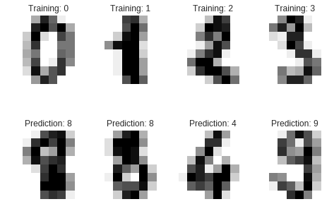
Digits Dataset
sklearn modeling
https://scikit-learn.org/stable/auto_examples/classification/plot_digits_classification.html
# Standard scientific Python imports
import matplotlib.pyplot as plt
# Import datasets, classifiers and performance metrics
from sklearn import datasets, svm, metrics
# The digits dataset
digits = datasets.load_digits()
# The data that we are interested in is made of 8x8 images of digits, let's
# have a look at the first 4 images, stored in the `images` attribute of the
# dataset. If we were working from image files, we could load them using
# matplotlib.pyplot.imread. Note that each image must have the same size. For these
# images, we know which digit they represent: it is given in the 'target' of
# the dataset.
images_and_labels = list(zip(digits.images, digits.target))
for index, (image, label) in enumerate(images_and_labels[:4]):
plt.subplot(2, 4, index + 1)
plt.axis('off')
plt.imshow(image, cmap=plt.cm.gray_r, interpolation='nearest')
plt.title('Training: %i' % label)
# To apply a classifier on this data, we need to flatten the image, to
# turn the data in a (samples, feature) matrix:
n_samples = len(digits.images)
data = digits.images.reshape((n_samples, -1))
# Create a classifier: a support vector classifier
classifier = svm.SVC(gamma=0.001)
# We learn the digits on the first half of the digits
classifier.fit(data[:n_samples // 2], digits.target[:n_samples // 2])
# Now predict the value of the digit on the second half:
expected = digits.target[n_samples // 2:]
predicted = classifier.predict(data[n_samples // 2:])
print("Classification report for classifier %s:\n%s\n"
% (classifier, metrics.classification_report(expected, predicted)))
print("Confusion matrix:\n%s" % metrics.confusion_matrix(expected, predicted))
images_and_predictions = list(zip(digits.images[n_samples // 2:], predicted))
for index, (image, prediction) in enumerate(images_and_predictions[:4]):
plt.subplot(2, 4, index + 5)
plt.axis('off')
plt.imshow(image, cmap=plt.cm.gray_r, interpolation='nearest')
plt.title('Prediction: %i' % prediction)
plt.show()
Classification report for classifier SVC(C=1.0, cache_size=200, class_weight=None, coef0=0.0,
decision_function_shape='ovr', degree=3, gamma=0.001, kernel='rbf',
max_iter=-1, probability=False, random_state=None, shrinking=True,
tol=0.001, verbose=False):
precision recall f1-score support
0 1.00 0.99 0.99 88
1 0.99 0.97 0.98 91
2 0.99 0.99 0.99 86
3 0.98 0.87 0.92 91
4 0.99 0.96 0.97 92
5 0.95 0.97 0.96 91
6 0.99 0.99 0.99 91
7 0.96 0.99 0.97 89
8 0.94 1.00 0.97 88
9 0.93 0.98 0.95 92
micro avg 0.97 0.97 0.97 899
macro avg 0.97 0.97 0.97 899
weighted avg 0.97 0.97 0.97 899
Confusion matrix:
[[87 0 0 0 1 0 0 0 0 0]
[ 0 88 1 0 0 0 0 0 1 1]
[ 0 0 85 1 0 0 0 0 0 0]
[ 0 0 0 79 0 3 0 4 5 0]
[ 0 0 0 0 88 0 0 0 0 4]
[ 0 0 0 0 0 88 1 0 0 2]
[ 0 1 0 0 0 0 90 0 0 0]
[ 0 0 0 0 0 1 0 88 0 0]
[ 0 0 0 0 0 0 0 0 88 0]
[ 0 0 0 1 0 1 0 0 0 90]]
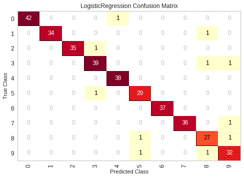
Yellowbrick Confusion Matrix
http://www.scikit-yb.org/en/latest/api/classifier/confusion_matrix.html
from sklearn.datasets import load_digits
from sklearn.model_selection import train_test_split
from sklearn.linear_model import LogisticRegression
from yellowbrick.classifier import ConfusionMatrix
# We'll use the handwritten digits data set from scikit-learn.
# Each feature of this dataset is an 8x8 pixel image of a handwritten number.
# Digits.data converts these 64 pixels into a single array of features
digits = load_digits()
X = digits.data
y = digits.target
X_train, X_test, y_train, y_test = train_test_split(X, y, test_size =0.2, random_state=1)
model = LogisticRegression()
# The ConfusionMatrix visualizer taxes a model
cm = ConfusionMatrix(model, classes=[0,1,2,3,4,5,6,7,8,9])
# Fit fits the passed model. This is unnecessary if you pass the visualizer a pre-fitted model
cm.fit(X_train, y_train)
# To create the ConfusionMatrix, we need some test data. Score runs predict() on the data
# and then creates the confusion_matrix from scikit-learn.
cm.score(X_test, y_test)
# How did we do?
cm.poof()
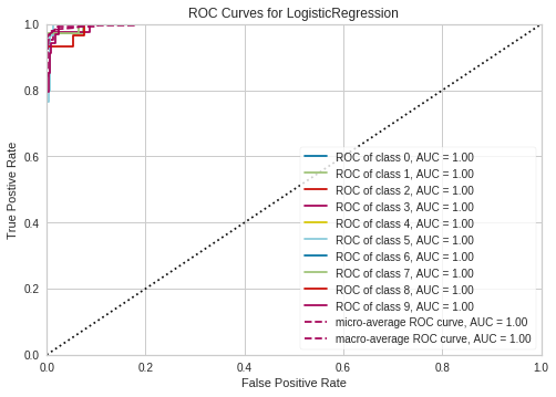
ROCAUC
http://www.scikit-yb.org/en/latest/api/classifier/rocauc.html
from yellowbrick.classifier import ROCAUC
from sklearn.linear_model import LogisticRegression
model = LogisticRegression()
classes=[0,1,2,3,4,5,6,7,8,9]
# Instantiate the visualizer with the classification model
visualizer = ROCAUC(model, classes=classes)
visualizer.fit(X_train, y_train) # Fit the training data to the visualizer
visualizer.score(X_test, y_test) # Evaluate the model on the test data
g = visualizer.poof() # Draw/show/poof the data
Supervized Machine Learning: Regression Modeling Workflow
Ingest
Source: http://wiki.stat.ucla.edu/socr/index.php/SOCR_Data_MLB_HeightsWeights
import pandas as pd
df = pd.read_csv("https://raw.githubusercontent.com/noahgift/functional_intro_to_python/master/data/mlb_weight_ht.csv")
df.head()
| Name | Team | Position | Height(inches) | Weight(pounds) | Age | |
|---|---|---|---|---|---|---|
| 0 | Adam_Donachie | BAL | Catcher | 74 | 180.0 | 22.99 |
| 1 | Paul_Bako | BAL | Catcher | 74 | 215.0 | 34.69 |
| 2 | Ramon_Hernandez | BAL | Catcher | 72 | 210.0 | 30.78 |
| 3 | Kevin_Millar | BAL | First_Baseman | 72 | 210.0 | 35.43 |
| 4 | Chris_Gomez | BAL | First_Baseman | 73 | 188.0 | 35.71 |
Find N/A
df.shape
(1034, 6)
df.isnull().values.any()
True
df = df.dropna()
df.isnull().values.any()
False
df.shape
(1033, 6)
Clean
df.rename(index=str,
columns={"Height(inches)": "Height", "Weight(pounds)": "Weight"},
inplace=True)
df.head()
| Name | Team | Position | Height | Weight | Age | |
|---|---|---|---|---|---|---|
| 0 | Adam_Donachie | BAL | Catcher | 74 | 180.0 | 22.99 |
| 1 | Paul_Bako | BAL | Catcher | 74 | 215.0 | 34.69 |
| 2 | Ramon_Hernandez | BAL | Catcher | 72 | 210.0 | 30.78 |
| 3 | Kevin_Millar | BAL | First_Baseman | 72 | 210.0 | 35.43 |
| 4 | Chris_Gomez | BAL | First_Baseman | 73 | 188.0 | 35.71 |
EDA
df.describe()
| Height | Weight | Age | |
|---|---|---|---|
| count | 1033.000000 | 1033.000000 | 1033.000000 |
| mean | 73.698935 | 201.689255 | 28.737648 |
| std | 2.306330 | 20.991491 | 4.322298 |
| min | 67.000000 | 150.000000 | 20.900000 |
| 25% | 72.000000 | 187.000000 | 25.440000 |
| 50% | 74.000000 | 200.000000 | 27.930000 |
| 75% | 75.000000 | 215.000000 | 31.240000 |
| max | 83.000000 | 290.000000 | 48.520000 |
Model
from sklearn import linear_model
from sklearn.model_selection import train_test_split
Create Features
var = df['Weight'].values
var.shape
(1033,)
y = df['Weight'].values #Target
y = y.reshape(-1, 1)
X = df['Height'].values #Feature(s)
X = X.reshape(-1,1)
#X = df[['Height', 'Age']].values
y.shape
(1033, 1)
Split data
X_train, X_test, y_train, y_test = train_test_split(X, y, test_size=0.2)
print(X_train.shape, y_train.shape)
print(X_test.shape, y_test.shape)
(826, 1) (826, 1)
(207, 1) (207, 1)
Fit the model
lm = linear_model.LinearRegression()
model = lm.fit(X_train, y_train)
predictions = lm.predict(X_test)
lm.predict?
Returns Numpy Array
type(predictions)
numpy.ndarray
Plot Predictions
from matplotlib import pyplot as plt
plt.scatter(y_test, predictions)
plt.xlabel("Actual Weight")
plt.ylabel("Predicted Weight")
Text(0, 0.5, 'Predicted Weight')
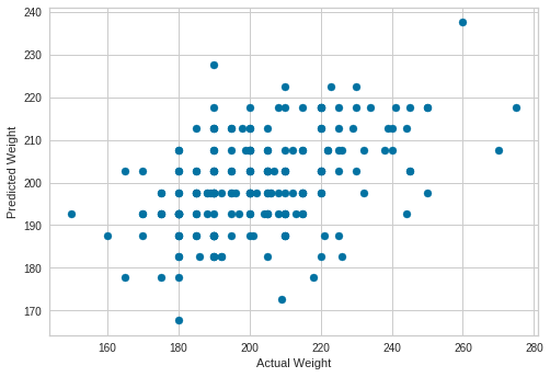
Print Accuracy of Linear Regression Model
model.score(X_test, y_test)
0.19307840892345418
Use Cross-Validation
from sklearn.model_selection import cross_val_score, cross_val_predict
from sklearn import metrics
scores = cross_val_score(model, X, y, cv=6)
scores
array([0.29670427, 0.22459508, 0.29543549, 0.30012566, 0.19191046,
0.34579806])
Plot Cross-validation Predictions
predictions = cross_val_predict(model, X, y, cv=6)
plt.scatter(y, predictions)
<matplotlib.collections.PathCollection at 0x7f6e32e91518>
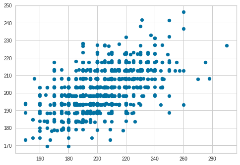
accuracy = metrics.r2_score(y, predictions)
accuracy
0.280770222008195
Conclusion
- Cross-Validation improved Accuracy
- Adding more data or more features could improve the model
- Major League Baseball may be a strange set to predict Weight
- Bigger Data Set here: http://socr.ucla.edu/docs/resources/SOCR_Data/SOCR_Data_Dinov_020108_HeightsWeights.html
Unsupervized Machine Learning: Clustering
Ingest
import pandas as pd
df = pd.read_csv(
"https://raw.githubusercontent.com/noahgift/food/master/data/features.en.openfoodfacts.org.products.csv")
df.drop(["Unnamed: 0", "exceeded", "g_sum", "energy_100g"], axis=1, inplace=True) #drop two rows we don't need
df = df.drop(df.index[[1,11877]]) #drop outlier
df.rename(index=str, columns={"reconstructed_energy": "energy_100g"}, inplace=True)
df.head()
| fat_100g | carbohydrates_100g | sugars_100g | proteins_100g | salt_100g | energy_100g | product | |
|---|---|---|---|---|---|---|---|
| 0 | 28.57 | 64.29 | 14.29 | 3.57 | 0.00000 | 2267.85 | Banana Chips Sweetened (Whole) |
| 2 | 57.14 | 17.86 | 3.57 | 17.86 | 1.22428 | 2835.70 | Organic Salted Nut Mix |
| 3 | 18.75 | 57.81 | 15.62 | 14.06 | 0.13970 | 1953.04 | Organic Muesli |
| 4 | 36.67 | 36.67 | 3.33 | 16.67 | 1.60782 | 2336.91 | Zen Party Mix |
| 5 | 18.18 | 60.00 | 21.82 | 14.55 | 0.02286 | 1976.37 | Cinnamon Nut Granola |
df.columns
Index(['fat_100g', 'carbohydrates_100g', 'sugars_100g', 'proteins_100g',
'salt_100g', 'energy_100g', 'product'],
dtype='object')
Create Features to Cluster
df_cluster_features = df.drop("product", axis=1)
Scale the data
from sklearn.preprocessing import MinMaxScaler
scaler = MinMaxScaler()
print(scaler.fit(df_cluster_features))
print(scaler.transform(df_cluster_features))
MinMaxScaler(copy=True, feature_range=(0, 1))
[[2.85700000e-01 6.42900000e-01 1.53063241e-01 6.89388819e-02
0.00000000e+00 5.06782123e-01]
[5.71400000e-01 1.78600000e-01 4.71343874e-02 2.06913199e-01
6.02500000e-04 6.33675978e-01]
[1.87500000e-01 5.78100000e-01 1.66205534e-01 1.70223038e-01
6.87500000e-05 4.36433520e-01]
...
[0.00000000e+00 1.33300000e-01 1.43577075e-01 3.44694410e-02
1.87500000e-05 5.06391061e-02]
[0.00000000e+00 1.62500000e-01 1.72430830e-01 3.44694410e-02
1.87500000e-05 6.17318436e-02]
[0.00000000e+00 0.00000000e+00 1.18577075e-02 3.44694410e-02
0.00000000e+00 0.00000000e+00]]
Add Cluster Labels
from sklearn.cluster import KMeans
k_means = KMeans(n_clusters=3)
kmeans = k_means.fit(scaler.transform(df_cluster_features))
df['cluster'] = kmeans.labels_
df.head()
| fat_100g | carbohydrates_100g | sugars_100g | proteins_100g | salt_100g | energy_100g | product | cluster | |
|---|---|---|---|---|---|---|---|---|
| 0 | 28.57 | 64.29 | 14.29 | 3.57 | 0.00000 | 2267.85 | Banana Chips Sweetened (Whole) | 2 |
| 2 | 57.14 | 17.86 | 3.57 | 17.86 | 1.22428 | 2835.70 | Organic Salted Nut Mix | 2 |
| 3 | 18.75 | 57.81 | 15.62 | 14.06 | 0.13970 | 1953.04 | Organic Muesli | 2 |
| 4 | 36.67 | 36.67 | 3.33 | 16.67 | 1.60782 | 2336.91 | Zen Party Mix | 2 |
| 5 | 18.18 | 60.00 | 21.82 | 14.55 | 0.02286 | 1976.37 | Cinnamon Nut Granola | 2 |
9.3 Learn pandas
Time Series Workflow
Ingest Zillow
import pandas as pd
pd.set_option('display.float_format', lambda x: '%.3f' % x)
import numpy as np
import statsmodels.api as sm
import statsmodels.formula.api as smf
import matplotlib.pyplot as plt
import seaborn as sns
import seaborn as sns; sns.set(color_codes=True)
from sklearn.cluster import KMeans
color = sns.color_palette()
from IPython.core.display import display, HTML
display(HTML("<style>.container { width:100% !important; }</style>"))
%matplotlib inline
df = pd.read_csv("https://raw.githubusercontent.com/noahgift/real_estate_ml/master/data/Zip_Zhvi_SingleFamilyResidence_2018.csv")
df.head()
| RegionID | RegionName | City | State | Metro | CountyName | SizeRank | 1996-04 | 1996-05 | 1996-06 | ... | 2018-03 | 2018-04 | 2018-05 | 2018-06 | 2018-07 | 2018-08 | 2018-09 | 2018-10 | 2018-11 | 2018-12 | |
|---|---|---|---|---|---|---|---|---|---|---|---|---|---|---|---|---|---|---|---|---|---|
| 0 | 84654 | 60657 | Chicago | IL | Chicago-Naperville-Elgin | Cook County | 1 | 334200.000 | 335400.000 | 336500.000 | ... | 1037400 | 1038700 | 1041500 | 1042800 | 1042900 | 1044400 | 1047800 | 1049700 | 1048300 | 1047900 |
| 1 | 91982 | 77494 | Katy | TX | Houston-The Woodlands-Sugar Land | Harris County | 2 | 210400.000 | 212200.000 | 212200.000 | ... | 330400 | 332700 | 334500 | 335900 | 337000 | 338300 | 338400 | 336900 | 336000 | 336500 |
| 2 | 84616 | 60614 | Chicago | IL | Chicago-Naperville-Elgin | Cook County | 3 | 498100.000 | 500900.000 | 503100.000 | ... | 1317900 | 1321100 | 1325300 | 1323800 | 1321200 | 1320700 | 1319500 | 1318800 | 1319700 | 1323300 |
| 3 | 93144 | 79936 | El Paso | TX | El Paso | El Paso County | 4 | 77300.000 | 77300.000 | 77300.000 | ... | 120800 | 121300 | 122200 | 123000 | 123600 | 124500 | 125600 | 126300 | 126800 | 127400 |
| 4 | 91940 | 77449 | Katy | TX | Houston-The Woodlands-Sugar Land | Harris County | 5 | 95400.000 | 95600.000 | 95800.000 | ... | 175500 | 176400 | 176900 | 176900 | 177300 | 178000 | 178500 | 179300 | 180200 | 180700 |
5 rows × 280 columns
EDA
df.describe()
| RegionID | RegionName | SizeRank | 1996-04 | 1996-05 | 1996-06 | 1996-07 | 1996-08 | 1996-09 | 1996-10 | ... | 2018-03 | 2018-04 | 2018-05 | 2018-06 | 2018-07 | 2018-08 | 2018-09 | 2018-10 | 2018-11 | 2018-12 | |
|---|---|---|---|---|---|---|---|---|---|---|---|---|---|---|---|---|---|---|---|---|---|
| count | 15508.000 | 15508.000 | 15508.000 | 14338.000 | 14338.000 | 14338.000 | 14338.000 | 14338.000 | 14338.000 | 14338.000 | ... | 15508.000 | 15508.000 | 15508.000 | 15508.000 | 15508.000 | 15508.000 | 15508.000 | 15508.000 | 15508.000 | 15508.000 |
| mean | 80789.618 | 47683.566 | 7754.500 | 115889.866 | 116007.379 | 116123.051 | 116235.493 | 116358.920 | 116501.681 | 116689.315 | ... | 279359.582 | 280672.685 | 282148.749 | 283446.447 | 284466.282 | 285500.200 | 286717.307 | 288029.320 | 289187.510 | 290106.635 |
| std | 31521.485 | 29008.034 | 4476.918 | 85115.825 | 85264.209 | 85413.118 | 85566.676 | 85744.243 | 85958.867 | 86230.630 | ... | 361868.364 | 361360.576 | 363102.089 | 365301.815 | 366277.876 | 367095.613 | 366772.521 | 364624.171 | 361143.146 | 359132.687 |
| min | 58196.000 | 1001.000 | 1.000 | 11300.000 | 11500.000 | 11600.000 | 11800.000 | 11800.000 | 12000.000 | 12100.000 | ... | 21700.000 | 21700.000 | 22100.000 | 22200.000 | 22000.000 | 21800.000 | 21700.000 | 21500.000 | 21600.000 | 21900.000 |
| 25% | 67215.000 | 22199.000 | 3877.750 | 66700.000 | 66800.000 | 66925.000 | 67100.000 | 67200.000 | 67300.000 | 67500.000 | ... | 128300.000 | 128800.000 | 129675.000 | 130300.000 | 131100.000 | 131900.000 | 132900.000 | 134000.000 | 135100.000 | 135600.000 |
| 50% | 77886.500 | 45792.500 | 7754.500 | 96500.000 | 96700.000 | 96750.000 | 96900.000 | 96900.000 | 97000.000 | 97150.000 | ... | 191100.000 | 192150.000 | 193400.000 | 194600.000 | 195700.000 | 196900.000 | 198100.000 | 199600.000 | 201100.000 | 202150.000 |
| 75% | 90314.250 | 74010.250 | 11631.250 | 140500.000 | 140600.000 | 140600.000 | 140800.000 | 141000.000 | 141100.000 | 141300.000 | ... | 310750.000 | 312300.000 | 314325.000 | 316100.000 | 317425.000 | 318325.000 | 319800.000 | 321200.000 | 322425.000 | 323900.000 |
| max | 753844.000 | 99901.000 | 15508.000 | 3676700.000 | 3704200.000 | 3729600.000 | 3754600.000 | 3781800.000 | 3813500.000 | 3849600.000 | ... | 17724700.000 | 17408900.000 | 17450500.000 | 17722800.000 | 18006700.000 | 18273800.000 | 18331900.000 | 18131900.000 | 17594900.000 | 17119600.000 |
8 rows × 276 columns
Clean Up DataFrame
Rename RegionName to ZipCode and Change Zip Code to String
df.rename(columns={"RegionName":"ZipCode"}, inplace=True)
df["ZipCode"]=df["ZipCode"].map(lambda x: "{:.0f}".format(x))
df["RegionID"]=df["RegionID"].map(lambda x: "{:.0f}".format(x))
df.head()
| RegionID | ZipCode | City | State | Metro | CountyName | SizeRank | 1996-04 | 1996-05 | 1996-06 | ... | 2018-03 | 2018-04 | 2018-05 | 2018-06 | 2018-07 | 2018-08 | 2018-09 | 2018-10 | 2018-11 | 2018-12 | |
|---|---|---|---|---|---|---|---|---|---|---|---|---|---|---|---|---|---|---|---|---|---|
| 0 | 84654 | 60657 | Chicago | IL | Chicago-Naperville-Elgin | Cook County | 1 | 334200.000 | 335400.000 | 336500.000 | ... | 1037400 | 1038700 | 1041500 | 1042800 | 1042900 | 1044400 | 1047800 | 1049700 | 1048300 | 1047900 |
| 1 | 91982 | 77494 | Katy | TX | Houston-The Woodlands-Sugar Land | Harris County | 2 | 210400.000 | 212200.000 | 212200.000 | ... | 330400 | 332700 | 334500 | 335900 | 337000 | 338300 | 338400 | 336900 | 336000 | 336500 |
| 2 | 84616 | 60614 | Chicago | IL | Chicago-Naperville-Elgin | Cook County | 3 | 498100.000 | 500900.000 | 503100.000 | ... | 1317900 | 1321100 | 1325300 | 1323800 | 1321200 | 1320700 | 1319500 | 1318800 | 1319700 | 1323300 |
| 3 | 93144 | 79936 | El Paso | TX | El Paso | El Paso County | 4 | 77300.000 | 77300.000 | 77300.000 | ... | 120800 | 121300 | 122200 | 123000 | 123600 | 124500 | 125600 | 126300 | 126800 | 127400 |
| 4 | 91940 | 77449 | Katy | TX | Houston-The Woodlands-Sugar Land | Harris County | 5 | 95400.000 | 95600.000 | 95800.000 | ... | 175500 | 176400 | 176900 | 176900 | 177300 | 178000 | 178500 | 179300 | 180200 | 180700 |
5 rows × 280 columns
median_prices = df.median()
#sf_prices = df["City"] == "San Francisco".median()
Median USA Prices December, 2018
median_prices.tail()
2018-08 196900.000
2018-09 198100.000
2018-10 199600.000
2018-11 201100.000
2018-12 202150.000
dtype: float64
sf_df = df[df["City"] == "San Francisco"].median()
df_comparison = pd.concat([sf_df,median_prices], axis=1)
df_comparison.columns = ["San Francisco","Median USA"]
df_comparison.tail()
| San Francisco | Median USA | |
|---|---|---|
| 2018-08 | 1828600.000 | 196900.000 |
| 2018-09 | 1823200.000 | 198100.000 |
| 2018-10 | 1823700.000 | 199600.000 |
| 2018-11 | 1813400.000 | 201100.000 |
| 2018-12 | 1806000.000 | 202150.000 |
Transpose
df_transposed = df.transpose()
df_transposed.head(15)
| 0 | 1 | 2 | 3 | 4 | 5 | 6 | 7 | 8 | 9 | ... | 15498 | 15499 | 15500 | 15501 | 15502 | 15503 | 15504 | 15505 | 15506 | 15507 | |
|---|---|---|---|---|---|---|---|---|---|---|---|---|---|---|---|---|---|---|---|---|---|
| RegionID | 84654 | 91982 | 84616 | 93144 | 91940 | 91733 | 61807 | 84640 | 62037 | 97564 | ... | 94711 | 62556 | 99032 | 62697 | 99074 | 58333 | 59107 | 75672 | 93733 | 95851 |
| ZipCode | 60657 | 77494 | 60614 | 79936 | 77449 | 77084 | 10467 | 60640 | 11226 | 94109 | ... | 84781 | 12429 | 97028 | 12720 | 97102 | 1338 | 3293 | 40404 | 81225 | 89155 |
| City | Chicago | Katy | Chicago | El Paso | Katy | Houston | New York | Chicago | New York | San Francisco | ... | Pine Valley | Esopus | Rhododendron | Bethel | Arch Cape | Buckland | Woodstock | Berea | Mount Crested Butte | Mesquite |
| State | IL | TX | IL | TX | TX | TX | NY | IL | NY | CA | ... | UT | NY | OR | NY | OR | MA | NH | KY | CO | NV |
| Metro | Chicago-Naperville-Elgin | Houston-The Woodlands-Sugar Land | Chicago-Naperville-Elgin | El Paso | Houston-The Woodlands-Sugar Land | Houston-The Woodlands-Sugar Land | New York-Newark-Jersey City | Chicago-Naperville-Elgin | New York-Newark-Jersey City | San Francisco-Oakland-Hayward | ... | St. George | Kingston | Portland-Vancouver-Hillsboro | NaN | Astoria | Greenfield Town | Claremont-Lebanon | Richmond-Berea | NaN | Las Vegas-Henderson-Paradise |
| CountyName | Cook County | Harris County | Cook County | El Paso County | Harris County | Harris County | Bronx County | Cook County | Kings County | San Francisco County | ... | Washington County | Ulster County | Clackamas County | Sullivan County | Clatsop County | Franklin County | Grafton County | Madison County | Gunnison County | Clark County |
| SizeRank | 1 | 2 | 3 | 4 | 5 | 6 | 7 | 8 | 9 | 10 | ... | 15499 | 15500 | 15501 | 15502 | 15503 | 15504 | 15505 | 15506 | 15507 | 15508 |
| 1996-04 | 334200.000 | 210400.000 | 498100.000 | 77300.000 | 95400.000 | 95000.000 | 152900.000 | 216500.000 | 162000.000 | 766000.000 | ... | 135900.000 | 78300.000 | 136200.000 | 62500.000 | 182600.000 | 94600.000 | 92700.000 | 57100.000 | 191100.000 | 176400.000 |
| 1996-05 | 335400.000 | 212200.000 | 500900.000 | 77300.000 | 95600.000 | 95200.000 | 152700.000 | 216700.000 | 162300.000 | 771100.000 | ... | 136300.000 | 78300.000 | 136600.000 | 62600.000 | 183700.000 | 94300.000 | 92500.000 | 57300.000 | 192400.000 | 176300.000 |
| 1996-06 | 336500.000 | 212200.000 | 503100.000 | 77300.000 | 95800.000 | 95400.000 | 152600.000 | 216900.000 | 162600.000 | 776500.000 | ... | 136600.000 | 78200.000 | 136800.000 | 62700.000 | 184800.000 | 94000.000 | 92400.000 | 57500.000 | 193700.000 | 176100.000 |
| 1996-07 | 337600.000 | 210700.000 | 504600.000 | 77300.000 | 96100.000 | 95700.000 | 152400.000 | 217000.000 | 163000.000 | 781900.000 | ... | 136900.000 | 78200.000 | 136800.000 | 62700.000 | 185800.000 | 93700.000 | 92200.000 | 57700.000 | 195000.000 | 176000.000 |
| 1996-08 | 338500.000 | 208300.000 | 505500.000 | 77400.000 | 96400.000 | 95900.000 | 152300.000 | 217100.000 | 163400.000 | 787300.000 | ... | 137100.000 | 78100.000 | 136700.000 | 62700.000 | 186700.000 | 93400.000 | 92100.000 | 58000.000 | 196300.000 | 175900.000 |
| 1996-09 | 339500.000 | 205500.000 | 505700.000 | 77500.000 | 96700.000 | 96100.000 | 152000.000 | 217200.000 | 164000.000 | 793000.000 | ... | 137400.000 | 78000.000 | 136600.000 | 62600.000 | 187700.000 | 93200.000 | 91900.000 | 58200.000 | 197700.000 | 175800.000 |
| 1996-10 | 340400.000 | 202500.000 | 505300.000 | 77600.000 | 96800.000 | 96200.000 | 151800.000 | 217500.000 | 164700.000 | 799100.000 | ... | 137700.000 | 78000.000 | 136400.000 | 62500.000 | 188700.000 | 93000.000 | 91700.000 | 58400.000 | 199100.000 | 175800.000 |
| 1996-11 | 341300.000 | 199800.000 | 504200.000 | 77700.000 | 96800.000 | 96100.000 | 151600.000 | 217900.000 | 165700.000 | 805800.000 | ... | 137900.000 | 78000.000 | 136000.000 | 62400.000 | 189800.000 | 92900.000 | 91300.000 | 58700.000 | 200700.000 | 176000.000 |
15 rows × 15508 columns
Create Cities DataFrame
cities = df_transposed.iloc[2].values
cities_df = df_transposed.drop(df_transposed.index[:7])
cities_df.columns = cities
cities_df.head()
| Chicago | Katy | Chicago | El Paso | Katy | Houston | New York | Chicago | New York | San Francisco | ... | Pine Valley | Esopus | Rhododendron | Bethel | Arch Cape | Buckland | Woodstock | Berea | Mount Crested Butte | Mesquite | |
|---|---|---|---|---|---|---|---|---|---|---|---|---|---|---|---|---|---|---|---|---|---|
| 1996-04 | 334200.000 | 210400.000 | 498100.000 | 77300.000 | 95400.000 | 95000.000 | 152900.000 | 216500.000 | 162000.000 | 766000.000 | ... | 135900.000 | 78300.000 | 136200.000 | 62500.000 | 182600.000 | 94600.000 | 92700.000 | 57100.000 | 191100.000 | 176400.000 |
| 1996-05 | 335400.000 | 212200.000 | 500900.000 | 77300.000 | 95600.000 | 95200.000 | 152700.000 | 216700.000 | 162300.000 | 771100.000 | ... | 136300.000 | 78300.000 | 136600.000 | 62600.000 | 183700.000 | 94300.000 | 92500.000 | 57300.000 | 192400.000 | 176300.000 |
| 1996-06 | 336500.000 | 212200.000 | 503100.000 | 77300.000 | 95800.000 | 95400.000 | 152600.000 | 216900.000 | 162600.000 | 776500.000 | ... | 136600.000 | 78200.000 | 136800.000 | 62700.000 | 184800.000 | 94000.000 | 92400.000 | 57500.000 | 193700.000 | 176100.000 |
| 1996-07 | 337600.000 | 210700.000 | 504600.000 | 77300.000 | 96100.000 | 95700.000 | 152400.000 | 217000.000 | 163000.000 | 781900.000 | ... | 136900.000 | 78200.000 | 136800.000 | 62700.000 | 185800.000 | 93700.000 | 92200.000 | 57700.000 | 195000.000 | 176000.000 |
| 1996-08 | 338500.000 | 208300.000 | 505500.000 | 77400.000 | 96400.000 | 95900.000 | 152300.000 | 217100.000 | 163400.000 | 787300.000 | ... | 137100.000 | 78100.000 | 136700.000 | 62700.000 | 186700.000 | 93400.000 | 92100.000 | 58000.000 | 196300.000 | 175900.000 |
5 rows × 15508 columns
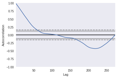
Create time series
from pandas.plotting import autocorrelation_plot
sf_values = cities_df.iloc[:, 9].values
index = pd.DatetimeIndex(cities_df.index.values)
sf_data = pd.Series(sf_values, index=index)
autocorrelation plot
Reference: https://pandas.pydata.org/pandas-docs/stable/user_guide/visualization.html#visualization-autocorrelation
autocorrelation_plot(sf_data)
<matplotlib.axes._subplots.AxesSubplot at 0x7f6e2fc637b8>
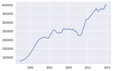
sf_data.tail()
2018-08-01 3993000
2018-09-01 3999000
2018-10-01 4014600
2018-11-01 4009500
2018-12-01 4016600
dtype: object
Simple Plot
sf_data.plot()
<matplotlib.axes._subplots.AxesSubplot at 0x7f6e32f078d0>
DataFrame Workflow
Ingest
import pandas as pd
df = pd.read_csv(
"https://raw.githubusercontent.com/noahgift/food/master/data/features.en.openfoodfacts.org.products.csv")
df.drop(["Unnamed: 0", "exceeded", "g_sum", "energy_100g"], axis=1, inplace=True) #drop two rows we don't need
df = df.drop(df.index[[1,11877]]) #drop outlier
df.rename(index=str, columns={"reconstructed_energy": "energy_100g"}, inplace=True)
df.head()
| fat_100g | carbohydrates_100g | sugars_100g | proteins_100g | salt_100g | energy_100g | product | |
|---|---|---|---|---|---|---|---|
| 0 | 28.570 | 64.290 | 14.290 | 3.570 | 0.000 | 2267.850 | Banana Chips Sweetened (Whole) |
| 2 | 57.140 | 17.860 | 3.570 | 17.860 | 1.224 | 2835.700 | Organic Salted Nut Mix |
| 3 | 18.750 | 57.810 | 15.620 | 14.060 | 0.140 | 1953.040 | Organic Muesli |
| 4 | 36.670 | 36.670 | 3.330 | 16.670 | 1.608 | 2336.910 | Zen Party Mix |
| 5 | 18.180 | 60.000 | 21.820 | 14.550 | 0.023 | 1976.370 | Cinnamon Nut Granola |
EDA
df.columns
Index(['fat_100g', 'carbohydrates_100g', 'sugars_100g', 'proteins_100g',
'salt_100g', 'energy_100g', 'product'],
dtype='object')
Rows and Attributes
df.shape
(45026, 7)
First Five Columns
df.head()
| fat_100g | carbohydrates_100g | sugars_100g | proteins_100g | salt_100g | energy_100g | product | |
|---|---|---|---|---|---|---|---|
| 0 | 28.570 | 64.290 | 14.290 | 3.570 | 0.000 | 2267.850 | Banana Chips Sweetened (Whole) |
| 2 | 57.140 | 17.860 | 3.570 | 17.860 | 1.224 | 2835.700 | Organic Salted Nut Mix |
| 3 | 18.750 | 57.810 | 15.620 | 14.060 | 0.140 | 1953.040 | Organic Muesli |
| 4 | 36.670 | 36.670 | 3.330 | 16.670 | 1.608 | 2336.910 | Zen Party Mix |
| 5 | 18.180 | 60.000 | 21.820 | 14.550 | 0.023 | 1976.370 | Cinnamon Nut Granola |
Descriptive Statistics
df.describe()
| fat_100g | carbohydrates_100g | sugars_100g | proteins_100g | salt_100g | energy_100g | |
|---|---|---|---|---|---|---|
| count | 45026.000 | 45026.000 | 45026.000 | 45026.000 | 45026.000 | 45026.000 |
| mean | 10.766 | 34.054 | 16.005 | 6.617 | 1.470 | 1111.286 |
| std | 14.930 | 29.557 | 21.496 | 7.926 | 12.795 | 791.609 |
| min | 0.000 | 0.000 | -1.200 | -3.570 | 0.000 | 0.000 |
| 25% | 0.000 | 7.440 | 1.570 | 0.000 | 0.064 | 334.520 |
| 50% | 3.170 | 22.390 | 5.880 | 4.000 | 0.635 | 1121.540 |
| 75% | 17.860 | 61.540 | 23.080 | 9.520 | 1.440 | 1678.460 |
| max | 100.000 | 100.000 | 100.000 | 100.000 | 2032.000 | 4475.000 |
Correlations
df.corr()
| fat_100g | carbohydrates_100g | sugars_100g | proteins_100g | salt_100g | energy_100g | |
|---|---|---|---|---|---|---|
| fat_100g | 1.000 | -0.051 | -0.068 | 0.383 | -0.003 | 0.768 |
| carbohydrates_100g | -0.051 | 1.000 | 0.669 | -0.097 | -0.011 | 0.580 |
| sugars_100g | -0.068 | 0.669 | 1.000 | -0.277 | -0.030 | 0.327 |
| proteins_100g | 0.383 | -0.097 | -0.277 | 1.000 | 0.016 | 0.391 |
| salt_100g | -0.003 | -0.011 | -0.030 | 0.016 | 1.000 | -0.007 |
| energy_100g | 0.768 | 0.580 | 0.327 | 0.391 | -0.007 | 1.000 |
Filtering by Quantiles
Find fatty foods in the 98th percentile
high_fat_df = df[df.fat_100g > df.fat_100g.quantile(.98)]
high_fat_text = high_fat_df['product'].values
len(high_fat_text)
878
high_fat_text[0]
'Organic Salted Nut Mix'
Find protein foods in the 98th percentile
high_protein_df = df[df.proteins_100g > df.proteins_100g.quantile(.98)]
high_protein_text = high_protein_df['product'].values
len(high_protein_text)
896
high_protein_text[0]
'Organic Yellow Split Peas'
9.4 Learn tensorflow
TensorFlow Hello World
References
- Official Hello World Example
- Adds two matrices
import tensorflow as tf
input1 = tf.ones((2, 3))
input2 = tf.reshape(tf.range(1, 7, dtype=tf.float32), (2, 3))
print("Two Tensor Flow Matrices with shape:")
print(input1.shape)
print(input2.shape)
Two Tensor Flow Matrices with shape:
(2, 3)
(2, 3)
output = input1 + input2
with tf.Session():
result = output.eval()
print("Result of addition of two Matrics")
result
Result of addition of two Matrics
array([[2., 3., 4.],
[5., 6., 7.]], dtype=float32)
9.5 Use seaborn for 2D plots
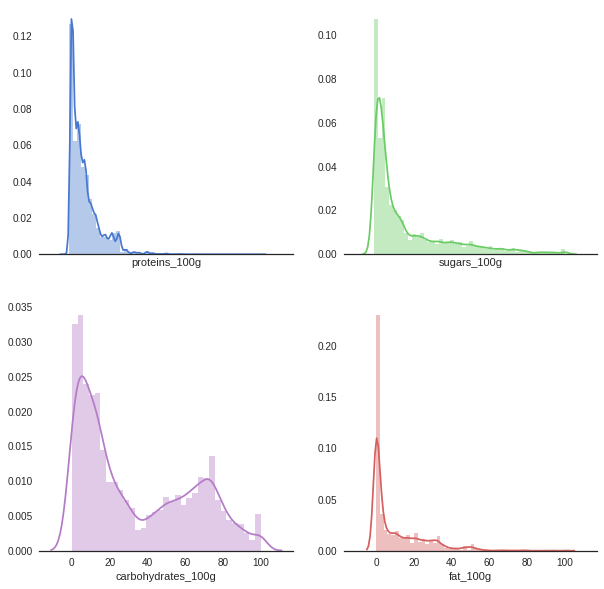
Faceted Distribution Plots
Generate distributions based on energy type
import seaborn as sns
import matplotlib.pyplot as plt
import warnings
import matplotlib.cbook
warnings.filterwarnings("ignore",category=matplotlib.cbook.mplDeprecation)
sns.set(style="white", palette="muted", color_codes=True)
# Set up the matplotlib figure
f, axes = plt.subplots(2, 2, figsize=(10, 10), sharex=True)
sns.despine(left=True)
# Plot each distribution on the 4 points
sns.distplot(df.proteins_100g, color="b", ax=axes[0, 0])
sns.distplot(df.sugars_100g, color="g", ax=axes[0, 1])
sns.distplot(df.fat_100g, color="r", ax=axes[1, 1])
sns.distplot(df.carbohydrates_100g, color="m", ax=axes[1, 0])
<matplotlib.axes._subplots.AxesSubplot at 0x7f59f80c4550>
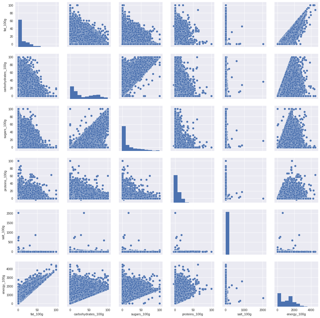
Pairplot
import seaborn as sns
sns.pairplot(df)
<seaborn.axisgrid.PairGrid at 0x7fd6031d4630>
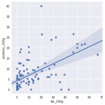
lmplot
import seaborn as sns
sns.lmplot(x="fat_100g", y="proteins_100g", data=df.sample(100))
<seaborn.axisgrid.FacetGrid at 0x7f6e135ab048>
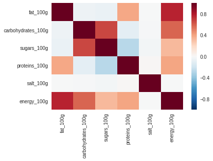
heatmap
sns.heatmap(df.corr())
<matplotlib.axes._subplots.AxesSubplot at 0x7f6e13550588>
9.6 Use Plotly for interactive plots
2D Plots
def enable_plotly_in_cell():
import IPython
from plotly.offline import init_notebook_mode
display(IPython.core.display.HTML('''
<script src="/static/components/requirejs/require.js"></script>
'''))
init_notebook_mode(connected=False)
from plotly.offline import init_notebook_mode
enable_plotly_in_cell()
init_notebook_mode(connected=False)
import cufflinks as cf
cf.go_offline()
df.sample(1000).iplot(kind='bubble',
size='energy_100g',
mode='markers',
x='fat_100g',
y='proteins_100g',
xTitle='Fat',
yTitle='Protein',
text="product")
3D ClusterPlot
Protein-Fat-Carb 3D Plot
import plotly.offline as py
import plotly.graph_objs as go
from plotly.offline import init_notebook_mode
enable_plotly_in_cell()
trace1 = go.Scatter3d(
x=df["fat_100g"],
y=df["carbohydrates_100g"],
z=df["proteins_100g"],
mode='markers',
text=df["product"],
marker=dict(
size=12,
color=df["cluster"], # set color to an array/list of desired values
colorscale='Viridis', # choose a colorscale
opacity=0.8
)
)
#print(trace1)
data = [trace1]
layout = go.Layout(
showlegend=False,
title="Protein-Fat-Carb: Food Energy Types",
scene = dict(
xaxis = dict(title='X: Fat Content-100g'),
yaxis = dict(title="Y: Carbohydrate Content-100g"),
zaxis = dict(title="Z: Protein Content-100g"),
),
width=1000,
height=900,
)
fig = go.Figure(data=data, layout=layout)
py.iplot(fig, filename='3d-scatter-colorscale')
Sugar-Salt-Carb-3D Plot
import plotly.offline as py
import plotly.graph_objs as go
from plotly.offline import init_notebook_mode
enable_plotly_in_cell()
trace1 = go.Scatter3d(
x=df["sugars_100g"],
y=df["carbohydrates_100g"],
z=df["salt_100g"],
mode='markers',
text=df["product"],
marker=dict(
size=12,
color=df["cluster"], # set color to an array/list of desired values
colorscale='Viridis', # choose a colorscale
opacity=0.8
)
)
#print(trace1)
data = [trace1]
layout = go.Layout(
showlegend=False,
title="Sugar, Carb, Salt: Food Energy Types",
scene = dict(
xaxis = dict(title='X: Sugar Content-100g'),
yaxis = dict(title="Y: Carbohydrate Content-100g"),
zaxis = dict(title="Z: Salt Content-100g"),
),
width=1000,
height=900,
)
fig = go.Figure(data=data, layout=layout)
py.iplot(fig, filename='3d-scatter-colorscale')
9.7 Specialized Visualization Libraries
Yellowbrick
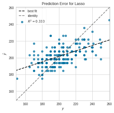
Visualize Regression Lasso (Regression) Model Accuracy with Yellowbrick
Note, uses Lasso Regression
from yellowbrick.regressor import PredictionError
from sklearn.linear_model import Lasso
lasso = Lasso()
visualizer = PredictionError(lasso)
visualizer.fit(X_train, y_train) # Fit the training data to the visualizer
visualizer.score(X_test, y_test) # Evaluate the model on the test data
g = visualizer.poof() # Draw/show/poof the data
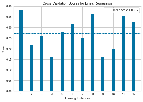
Visualize cross-validated scores for Linear regression model
See this: http://www.scikit-yb.org/en/latest/api/model_selection/cross_validation.html
from sklearn.linear_model import Ridge
from sklearn.model_selection import KFold
from yellowbrick.model_selection import CVScores
# Create a new figure and axes
_, ax = plt.subplots()
cv = KFold(12)
oz = CVScores(
linear_model.LinearRegression(), ax=ax, cv=cv, scoring='r2'
)
oz.fit(X, y)
oz.poof()
Word Cloud
from wordcloud import WordCloud, STOPWORDS
import matplotlib.pyplot as plt
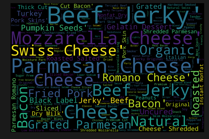
High protein foods
Find protein foods in the 98th percentile
high_protein_df = df[df.proteins_100g > df.proteins_100g.quantile(.98)]
high_protein_text = high_protein_df['product'].values
len(high_protein_text)
896
Word Cloud High Protein
wordcloud = WordCloud(
width = 3000,
height = 2000,
background_color = 'black',
stopwords = STOPWORDS).generate(str(high_protein_text))
fig = plt.figure(
figsize = (10, 7),
facecolor = 'k',
edgecolor = 'k')
plt.imshow(wordcloud, interpolation = 'bilinear')
plt.axis('off')
plt.tight_layout(pad=0)
plt.show()
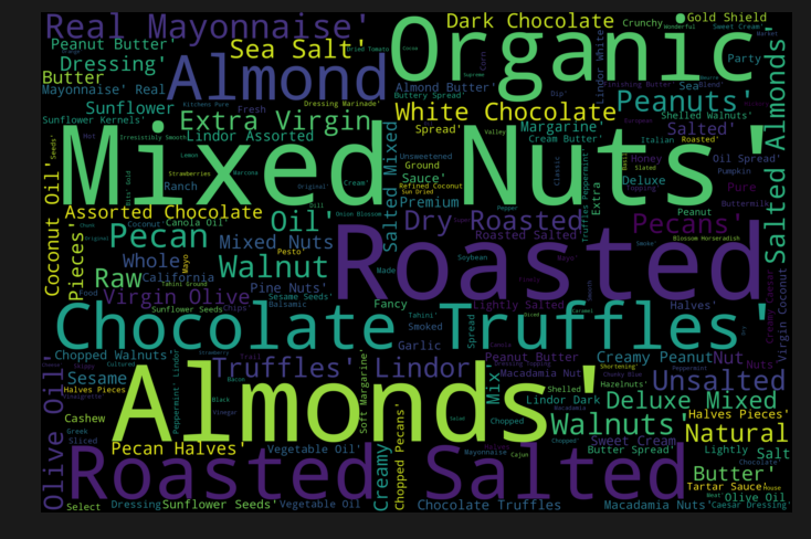
High fat foods
Find fatty foods in the 98th percentile
high_fat_df = df[df.fat_100g > df.fat_100g.quantile(.98)]
high_fat_text = high_fat_df['product'].values
len(high_fat_text)
878
Word Cloud High Fat
wordcloud = WordCloud(
width = 3000,
height = 2000,
background_color = 'black',
stopwords = STOPWORDS).generate(str(high_fat_text))
fig = plt.figure(
figsize = (10, 7),
facecolor = 'k',
edgecolor = 'k')
plt.imshow(wordcloud, interpolation = 'bilinear')
plt.axis('off')
plt.tight_layout(pad=0)
plt.show()
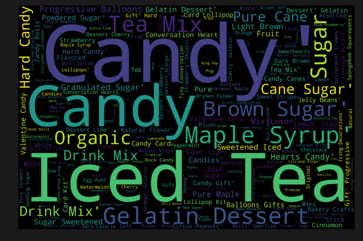
High sugar foods
Find sugary foods in the 98th percentile
high_sugar_df = df[df.sugars_100g > df.sugars_100g.quantile(.98)]
high_sugar_text = high_sugar_df['product'].values
len(high_sugar_text)
893
Word Cloud High Sugar
wordcloud = WordCloud(
width = 3000,
height = 2000,
background_color = 'black',
stopwords = STOPWORDS).generate(str(high_sugar_text))
fig = plt.figure(
figsize = (10, 7),
facecolor = 'k',
edgecolor = 'k')
plt.imshow(wordcloud, interpolation = 'bilinear')
plt.axis('off')
plt.tight_layout(pad=0)
plt.show()
9.8 Learn Natural Language Processing Libraries
NLTK Stopword Processing
Setup Stop Words
import nltk
from nltk.corpus import stopwords
nltk.download('stopwords')
stop = stopwords.words('english')
[nltk_data] Downloading package stopwords to /root/nltk_data...
[nltk_data] Unzipping corpora/stopwords.zip.
Preprocess Text
dataset = df['product'].fillna("").values
raw_text_data = [d.split() for d in dataset]
Remove stop words
text_data = [item for item in raw_text_data if item not in stop]
Gensim Topic Modeling
from gensim import corpora
dictionary = corpora.Dictionary(text_data)
corpus = [dictionary.doc2bow(text) for text in text_data]
import gensim
NUM_TOPICS = 5
ldamodel = gensim.models.ldamodel.LdaModel(
corpus, num_topics = NUM_TOPICS, id2word=dictionary, passes=15)
topics = ldamodel.print_topics(num_words=4)
for topic in topics:
print(topic)
(0, '0.039*"Chocolate" + 0.033*"Cream" + 0.030*"Milk" + 0.027*"Juice"')
(1, '0.030*"Fruit" + 0.023*"&" + 0.022*"Light" + 0.021*"Premium"')
(2, '0.087*"Cheese" + 0.028*"&" + 0.026*"Candy" + 0.023*"Cheddar"')
(3, '0.034*"In" + 0.032*"Sauce" + 0.029*"Sweet" + 0.025*"&"')
(4, '0.045*"Beans" + 0.037*"Mix" + 0.022*"Green" + 0.022*"&"')